last update 09/08/2006
2D/3D Real Time Object Tracking
Many imaging projects are based on the tracking of complete objects or markers on objects
in 2- or 3-dimensional space at high speed. The picCOLOR Real Time Position Tracking extension
module was developed to meet these requirements. The functions of this extension module allow
the automatic or interactive selection of markers and the set up of camera locations and
transformation equations for reconstruction of 3-dimensional coordinates from two camera views.
Usually the speed of the analysis is a very important question. The functions of the
extension module are optimized to run at highest possible speed for real-time applications.
Depending on the type of video camera, high tracking frequencies can be realised. With a
simple CCIR camera, a 3-dimensional tracking frequency of 25 Hz is possible. For higher
speed requirements special CMOS cameras can be used at tracking speed of up to 1000 Hz for
3-dimensional tracking. Of course the functions of the extension module can also be
used for post-processing of already loaded or recorded video sequences or single frames.
A few words on "real time": "real time" is a widely used - or misused - term in modern high
speed computing. What does it mean? Does it mean to finish a certain calculation extremely
fast, or analyse extremely quick events? - Not at all: "real time" just means to analyse an event
at exactly the time as it is taking place in reality, may it be slow or fast. This enables the
software (or the user) to react on a special event or to control a process in timely manner.
Therefore, the first thing to do in a real time task is to define or find out
how fast a process is going to happen and how fast a reaction must be to be able to perform
any control function. An often used definition is "video real time". Regular video frequency is
25Hz for European CCIR video standard. If a process can not be dissolved at this frequency,
like for instance a high frequency aircraft wing model flutter problem, a special high speed
camera has to be used. On the other hand there are many processes that are a lot slower
than video frequency. An example for this is the global adjustment of the angle of attack of
an aircraft model in the windtunnel. An analysis in video real time would normally be
nonsense for such tasks. Instead, an analysis of one frame per second seems sufficient for a
normal measurement procedure. Still this would be a "real time" control task. Usually, however,
real time tasks have a requirement for extremely high computing power and optimal programming:
all functions have to be optimized for certain tasks. Please call the picCOLOR development team
for information on special functions and solutions.
Marker Tracking
In the actual program version, markers can be any distinguishable areas on the surface that are
detectable by their gray level, dark or bright. These may be little pieces of paint or adhesive
tape, or little light bulbs or LED’s. The center of the markers will be determined at sub-pixel
accuracy by measuring the center of gravity of the pixel area. Of course the markers should not
change their geometry too much when viewed from different angles. An accuracy of 1/10 pixel length
can be achieved when the markers have at least a diameter of approximately 10 pixel. Smaller marker
diameters increase the processing speed, while larger markers result in higher resolution of
the detected coordinates. In a future version of the program, pattern matching algorithms will
be used to enable the usage of even more complex markers.
The resolution of the tracking depends on the object/marker size, on camera resolution, and
on camera arrangement. Regular CCIR video cameras have a resolution of 768*576 pixel. At the
optimum subpixel resolution of 1/10 pixel a resolution of approximately 7680 units per image
is possible in horizontal direction. Higher resolution cameras can be used, for example 4 Megapixel
cameras at 2048*2048 pixels for an approximate 20480 unit resolution. For 3-dimensional tracking
the resolution also depends on the arrangement of the cameras. A larger stereo angle is better for
higher depth resolution. Actual resolution can be determined from conversion of the pixel
units to real space dimensions. If, for instance, images of 1000 mm horizontal extension are
acquired using the 4 Megapixel camera, the horizontal 2-dimensional resolution would be approximately
0.05 mm. 3D-reconstruction will reduce this by a factor of sqrt(2) to a theoretical optimal
3D-resolution of 0.07mm. Surface deflection measurements like twist angles of aircraft wings,
measured by taking two marker locations at leading and trailing edge, may have a resolution of
some 0.056 degree, for the above example with a marker distance over the wing chord of 100mm.
Regression or avering over several marker pairs can increase the resolution. Of course there are
many influences and boundary conditions as well that may reduce the accuracy further. These
could be lens distortions, electronic image noise, calibration problems, and others.
The arrangement of the measurement system is very simple, just set up two or more cameras
for a 3D-measurement, define some reference positions by using a known set of
reference points, let the system calculate transformation matrices for a 3-dimensional
reconstruction, check the reconstruction using the known reference points, and start the
measurement. If 6 or more reference points are known, then not even the camera positions have
to be determined as the system can determine them from the 12 or more images of these points
in the two camera views. Results can be output as 3D-coordinates of all marker points or as
translations and rotations of the complete object as it is defined by the marker points.
Output data can be send to other programm applications on the same computer or to other
computer systems via software (TCP/IP, Microsoft DDE) of hardware (serial/parallel I/O).
The detected positions of the markers can be used to control any hardware. This could be a
model support control unit in a windtunnel or any other device that is controllable by a
computer.
Marker Tracking Parameters
Marker tracking parameters can be set up in a dialog box of the picCOLOR program with following selections:
- Set a useful length unit to calibrate the system, like Meters [m], or Inches [in].
- Acquire or load reference image (or two images for 3D) with markers in reference positions.
- Estimate approximate diameter of markers (in pixel size) with the mouse pointer
- Open the "Object Tracking Parameters" dialog box and define the following settings:
- Number of markers to be searched (count all marker images in case of two camera views)
- Set approximate diameter of the markers (all markers should have similar - not too much
more than factor 2 - diameter for this software version)
- Select a simple 2-dimensional detection or a 3-dimensional reconstruction. In case of a 3-
dimensional reconstruction select the split-screen mode or the two-screen mode. Depending
on the hardware, the screen can be split vertically or horizontally, as defined in the "Split-
Screen"-menu in the "Acquire"-menu. For two-screen mode select an additional image buffer
for the second view.
- Define the maximum allowable pixel-shift of the markers from one image to the next one in
the sequence. If the marker will move more than by this value within one frame time step,
the marker can not be found anymore and an error condition will be shown.
- Set marker validation: This is used to ensure the recognition of the correct marker images.
This recognition is based on overall pixel area or other features of the markers. Markers are
rejected if any of the selected rejection criteria are not met. There are individual or global
rejection criteria.
- Lost marker extrapolation: Markers can be tracked even if they are covered or hidden by other
objects. To do this, either the last savely determined marker speed and direction is used, or
the marker location is reconstructed using the nearest neighbors. When the marker reappears,
a recognition and reattachment is quite savely done. Turn this off for chaotically moving markers
or for very flexible surfaces where the nearest neighbor markers have no connection to the
hidden marker.
- Automatic Adaption to Light Conditions: Select this functionality, if the illumination conditions
will change a lot during measurement time and the system will automatically adapt thresholds to the
changing gray levels.
- Now define the marker positions by clicking the center of the markers with the left mouse
button. For a 3-dimensional reconstruction the markers in both stereo images have to be
defined in the same order. Otherwise an attachment of the correct markers in both images is
not possible. After this initialization a 2-dimensional tracking can be startet immediately.
For a 3-dimensional tracking the reconstruction parameters have to be initialized before any
measurement as explained below.
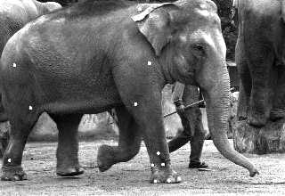

Fig.1,2: Example: Tracking of the joint positions of large mammals for investigation of motion physics

Fig.3,4: Motion of joint positions during fast walking / Hip joint motion during foot lift off
During tracking, an error code will be determined showing the status of the tracking for all
markers. Depending on the error code, the marker position may be unsave or completely
wrong. The control program receiving the positions and the error code can react usefully
when evaluating the error code. The following codes are implemented in the actual software:
- 0: marker correctly detected, positions are save.
- 1: marker detected to be close to the image border and may be leaving the image very soon, positions are save.
- 2: marker was reconstructed from neighbors, position should be save but probably less exact.
- 3: marker was rejected by any of the selected geometric or gray level rejection criteria.
- 4: marker touches the border of the search rectangle, i.e. marker has moved to much within one frame time step.
- 5: marker not found.
- 6: found more than one possible marker in the search rectangle.
- 7: 3D reconstruction problem.
Do not use positions if error codes are 3 or higher.
3D-Reconstruction
If positions of two cameras and their optical characteristics are known exactly, a 3-
dimensional reconstruction is very straight-forward. From two camera views of a certain
marker in 3-dimensional space its location can be determined by regarding the images as
result of certain translations and rotations and a final projection on the image plane. After
calculating transformation matrices for both cameras the transformation equations for each
marker image can be constructed, giving an over-defined equation system that can be
solved by a "least square"-method. A disadvantage of this direct method is the fact that
normally camera positions are not known very exactly. Especially the viewing angles and the
rotations about the optical axis of the cameras can only be measured approximately.
In this case a different approach can be used. The transformation matrices can be
determined without knowing the camera positions if at least 6 spatial reference points are known and
their images can be detected in both camera views. For each camera position a homogenous
system of at least 12 equation with 12 variables can be defined from which a system of
inhomogenous equations can be derived and solved by a Gauss-algorithm with post-iteration.
If more than the minimum of 6 reference points are provided, a Gauss approximation can be done
resulting in a set of error vectors for all calibration points. Accuracy is increased even
for non-exact reference positions and the quality of the calibration can be estimated.
After successfully calculating the transformation matrices, the 3-dimensional coordinates of
any other spatial points can be detected if their images can be found (tracked) in both
camera views. Additionally, a set of points can be defined as rigid object and the motion of
this object (translation and rotation) can be determined. Normal procedure of calibration and
initialization is outlined here:

Fig.5: Sketch of the 3D-Camera-Position dialog box
3D-Parameter Set-Up: Camera positions not known - using more than 6 reference points
- Input a useful system calibration unit: [m], [in] or other.
- Define the marker positions of the more than 6 known reference points in the two camera views
interactively by using the "Define Marker"-function. (After setting all usual marker parameters)
- Open "3D_CameraPosition"-dialog box and select "Least Square Reconstruction"
- Input the known reference points with x,y,z-coordinates in the selected calibration unit.
- Hit the "Transfer Marker" button to initialize internal variables.
- Determine the transformation matrices by hitting the "Calculate Matrices"-button.
- Check the transformation matrices by plotting the reference points as 2-dimensional
projections on the screen. They must fit exactly on the original marker images.

Fig.6: Sample reference object with 16 bright LED's at known 3D-points for reference and calibration

Fig.7: Same reference object with all points illuminated for automatic recognition by the software
Back to FIBUS Home Page
Back to Image Processing
Copyright © 2006 The
FIBUS Research Institute, Dr. Reinert H. G. Mueller;